kdb+: Joins for Beginners’

I was recently given the opportunity to learn kdb+ and, coming from a Sybase-flavoured SQL background, there were plenty of new concepts to learn. Some I was already familiar with – especially when it came to joins.

The joins I knew and loved so well from SQL were all available in kdb+, so they were easy to for me to get to grips with. However, there were a few new joins that I’d never heard of before, like the as-of join. These joins are especially powerful in the financial world, and it took me some time to wrap my head around them.

I decided to write a blog that a qbie like myself wished they had when they came to study kdb+ joins – with the help of visuals I hope this guide is useful for other qbies. I have also attached a basic summary of Joins here which you may enjoy reading also.

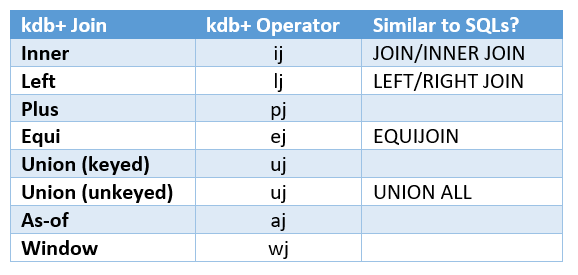
The table below shows the kdb+ joins that I will cover, as well as any SQL equivalent of the join (this is purely for reference, I will not be comparing exact like-for-like in this blog between kdb+ and SQL).

kdb+ Table Structure

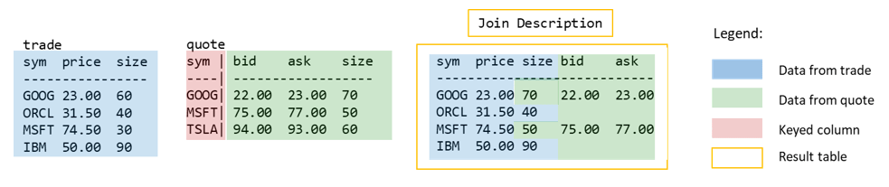
Below is a quick visual to describe how kdb+ tables are displayed on the console, and how they will be formatted throughout this blog:

This joins two tables based on the key column of the second table. The result has all the columns from table1, and any extra columns from table2 are appended on. The result table includes only combined rows from table1 and table2 where there are matching values in the common column that is keyed in table2, and it drops any rows that don’t.

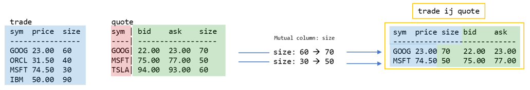
• schema of trade is kept, then any new columns from quote (‘bid’ and ‘ask’) are appended with their data
• any mutual columns (‘size’) will have quote’s data
• if any row’s value from trade does not exist in quote’s key, it will be dropped (i.e. in trade where sym=’ORCL’ and ‘IBM’)

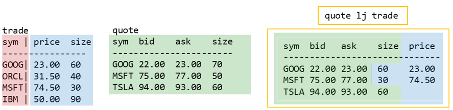
Left join takes two tables and joins them based on the key column of the second table. The result is all rows from table1 combined with either updated or additional data coming from table2. The result table always has the same row count as table1.

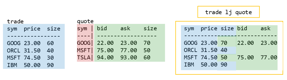
• the structure of trade is kept and additional columns from quote are joined on
• values from trade are overwritten by values from quote for the mutual column (‘size’) where there is a match on quote’s key (sym=’GOOG’ and ‘MSFT’)
• values from quote for columns ‘bid’ and ‘ask’ are joined where there is a match on quote’s key
• nulls are used to fill where there is no match on quote’s key (sym=’ORCL’ and ‘IBM’)
• the row from quote where sym=’TSLA’ is dropped as this value is unique to quote

The equivalent of SQL’s right join can be achieved by reversing the order of the tables in the left join:

The above image is how you would achieve SQLs “trade RIGHT JOIN quote” in kdb+. As you can see, SQL’s right join is just a left join in disguise!

This joins two tables based on the key column of the second table, and the result has the numerical values of unkeyed mutual columns added together.

• sums values from numerical columns between trade and quote
• the values from the mutual column ‘size’ have been added together
• if quote doesn’t have a matching numerical column to trade (e.g. ‘price’) it will replace the nulls with zeros
• if there are any mutual columns that are not a numerical type, plus join will try to add them which will throw a ‘type error

The equi join takes two tables and allows you to specify which mutual columns you want them to be joined on. The result combines all rows from table2 that match table1 on the specified columns.

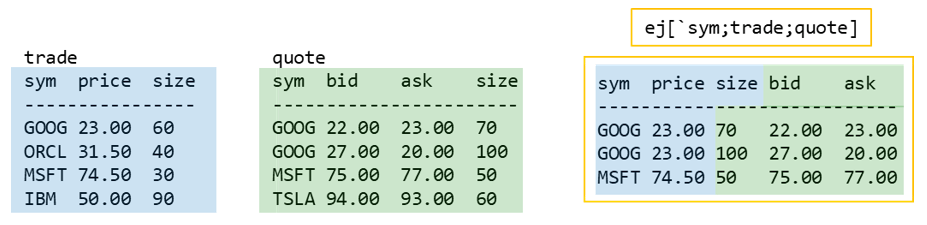
• the only syms that match between trade and quote are ‘GOOG’ and ‘MSFT’
• values are taken from quote for the mutual column to both tables (‘size’)
• two ‘GOOG’ rows are returned as there are two in quote
  • if an inner join was used, only the first ‘GOOG’ row from quote would be returned

Having any of the input tables keyed doesn’t make a difference to the output of equi join.

Union join combines all columns and rows from both tables. Common columns are merged, and new columns are appended and filled with nulls. The union join behaves differently depending on whether the tables are keyed, so let’s have a look at both…

Keyed uj

When tables are keyed, the matching rows are updated.

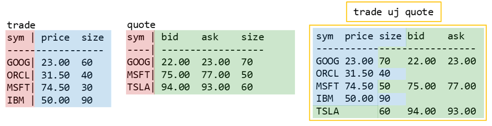
• ‘GOOG’ and ‘MSFT’ are keys in both tables, so the rows combine as shown
  • columns present in both tables take their values from quote (for ‘MSFT’, size=50 instead of 30)
• syms ‘ORCL’ and ‘IBM’ only exist in trade, and ‘TSLA’ only exists in quote, so they don’t have any updated values in the result
  • e.g. for sym=’ORCL’, the ‘bid’ column is filled with a null in the result set

Unkeyed uj

When tables are not keyed, the tables are simply appended to each other.

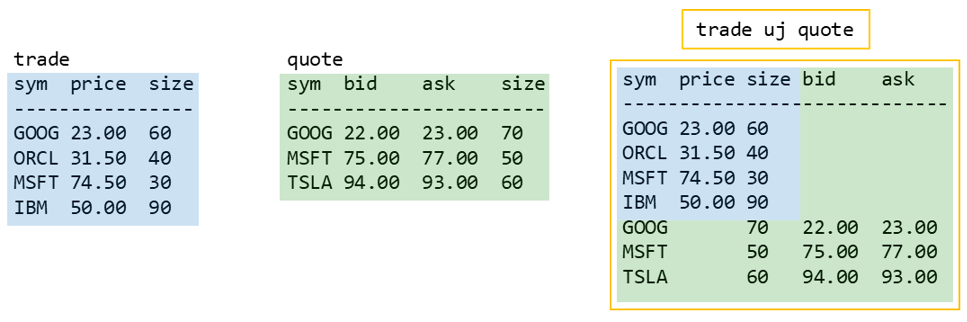
• result table has trade’s schema with any extra columns from quote appended
• values from trade are kept under their respective columns, with nulls filling new columns from quote (i.e. the ‘ask’ column)
• rows from quote are appended after the rows from trade, again with nulls used for non-mutual columns from trade (i.e. the ‘price’ column)

Working in capital markets I wondered where the new join concepts had been all my life. The as-of join and the window join which allow for non-equality-based matching are so useful on a day to day basis that I hope everyone can use this blog to harness their power. These joins have been so influential that the likes of Pandas, Apache Spark and R have implemented their own versions.

As-of Join

The as-of join matches two tables on a given column (e.g. sym) and returns the rows equal to or before another given column (e.g. time). The example below explains how it works.

There are many ways of using this join, but the most common is when you would like to know the latest quote on the market when a trade was done:

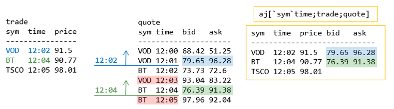
• result table contains all columns from trade and quote tables
• for VOD, it finds the last row from quote as-of the time of the trade (12:02), i.e. the last bid/ask at or before time 12:02
  • since there is no quote at 12:02, it joins the quote (bid/ask) from 12:01
  • this ignores where time is 12:03 in quote since this time is greater than 12:02
• for BT, finds the last quote as-of 12:04
  • however, this time there is a quote for that exact time, so it joins the bid/ask from 12:04
  • again, time at 12:05 in quote is ignored
• there is no quote for TSCO, so the bid and ask columns in the result are filled with null
• result will have the same shape as the trade table, adding new columns from quote (bid, ask)

Window Join

This joins two tables based on given columns, time intervals and an aggregate function effectively summarising t2s data.

The example below uses time intervals (or “windows”) of 2 seconds before and after each time in t1. The join then finds all sizes from t2 within each window (w) and averages them.

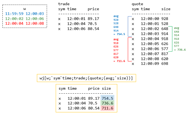
• for the first window (in blue), it finds 4 sizes in t2 within 11:59:59 and 12:00:03 that have an average of 754.5
• this same logic is repeated for the next 2 windows – (12:00:02-12:00:06 and 12:00:04-12:00:08)
• the results are joined on to each row of t1
  • you need to provide the same number of windows as there are rows in t1
• the last row of t2 is not included in the results as it lies outside of the window

As a qbie it took me a moment to grasp the syntax for the window intervals, so hopefully this helps!

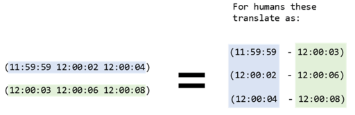
Window Join receives the window intervals as two lists. The first containing the list of start times and the second containing the list of end times:

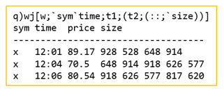
Tip! Use identity function :: in place of an aggregate function if you want all interval values returned.

Joins are the bread and butter of much of the high-level work you’ll do with kdb+. I hope through reading this guide you can spend less time learning and more time doing!